3. Cycles

3.1. Explanation of Cycles

We would usually think that constraint networks should not permit cycles, and for good reason. A cycle indicates that the value of a variable is dependent upon itself, an illogical proposition for a causal model.

However, there are many instances where variables might represent multiple values, such as a variable that varies in time. In this case each progressive value of the variable might be dependent upon previous values of itself. This kind of relationships can be modeled easily enough: just make a different node for every instance of a variable.

Note

The following example is modeled as a simple demo in the main package, available here.

Let’s say for example, that we wanted to solve for the position \(x\) of a car moving at constant velocity \(v\). The first step would be to set the starting position \(x_0\) and add it to the hypergraph. We can then add another node for the position after \(\Delta{}t\) seconds had gone by and call it \(x_1\). The relationship between \(x_1\) and \(x_0\) is \(x_1 = x_0 + v\Delta{}t\), which we can easily make into a hyperedge. We could repeat this process for the position after \(2\Delta{}t\) seconds had gone by, noting that \(x_2 = x_1 + v\Delta{}t\). This results in a drawn out hypergraph similar to the one shown in Figure 1.

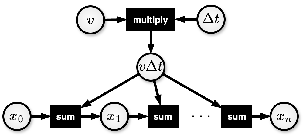
A simple hypergraph explicitly mapping out the relationships between variables.

Such a modeling process is not only tedious, it lacks expressability. What we really want to model is the relationship \(x_{i+1} = x_i + v\Delta{}t\), rather than every incremental relation. The trick for adding the variables \(x_i\) and \(x_{i+1}\) to the hypergraph is to use cycles.

Cycles enable arbitrary indexing of a variable, allowing us to express these recursive type expressions without have to explicitly map out every single instance of a variable, as shown in Figure 2.

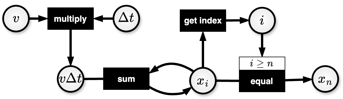
A non-simple hypergraph compressing Figure 1 with a cycle, where the cycle is terminated by a conditional edge when \(i \geq n\).

If you print the summary method on the above constraint hypergraph, you’ll get the following output:

└──x_n, index=1, cost=3
    ├◯─x, index=1, cost=2
    │  ├◯─x[CYCLE], index=1
    │  └●─delta_x, index=1, cost=1
    │     ├◯─velocity, index=1
    │     └●─delta_t, index=1
    └●─n, index=1

Note that the solver found the cycle, and highlighted it in the output.

3.2. Problems with Cycles

3.2.1. Representing Cycles

Representing cycles causes significant technical problems that have to be addressed. The first is that we need a way to identify which instance of a variable is being referenced in the graph, because \(x_1\) might be related to \(x_0\), but \(x_{308}\) is not! To do we introduce a index that allows us to note which version of a variable we’re dealing with. ConstraintHg will keep track of indices for us, but whenever we have a cycle (where a variable becomes dependent upon itself) we need to manually indicate the index to employ.

This occurs in the pendulum when we integrate the values (refer to the last two equations given at the beginning). In these cases, we have to indicate that the acceleration \(\alpha\) being solved for by the model is really \(alpha_{i+1}\). The way to do this is supplying the index_offset parameter to the add_edge function call. Go ahead and add index_offset=1 to the last edge in your script, so that the line looks like this:

hg.add_edge(
    sources={'F': F},
    target=alpha,
    rel=R.equal('F'),
    index_offset=1, # <- Add this line in
    label='F->alpha',
)

This indicates that the node alpha is constrained to be the value of the node F and that whenever this constraint is applied the index of alpha should be increased by one.

Important

To use a cycle, the solver needs a condition for exiting the cycle.

3.2.2. Cycle Complexity

Cycles can lead to highly complex simulations. Every iteration of a cycle forms it’s own path to an output, an includes all the previous paths as divergent possibilities. This means that the number of paths in a hypergraph grows factorially as a cycle is iterated over.

This can lead to dramatic chokepoints, to the point of making a system unsolveable. Every time the solver goes around the cycle it will have to consider all the previously solved values for \(\alpha\). Each of these values represents a unique path through the graph that must be advanced by the solver–after all, the solver doesn’t know which one of these paths will wind up being the one that ends up solving for the final node. However, because of the way we have our model set up, each value for \(\alpha\) gets used to solve for a new value of \(\theta\) and \(\omega\), creating new paths, each of which will result in the generation of two new values of \(\alpha\). If you do an analysis, the bifurcation results in the creation of \(n_i = n_{i-1}(n_{i-1} + 1)\) new paths for every \(i\)-th cycle we iterate through. The number of paths at each cycle are shown in the following table:

\(i\)	Paths (n)
0	1
1	2
2	6
3	42
4	1,806
5	3,263,442
6	10,650,056,950,806

This isn’t just exponential growth, it’s factorial exponential growth, growing in complexity so quickly that after just 8 cycles it outnumbers the number of atoms in the universe. Clearly this is untenable. However, we know that the vast majority of these branches are not going to be part of valid search path. Our solution to handling this complexity is to add additional information that helps the solver tame the expanding search space.

Typically when solving a cycle we only want to consider the most recently solved version of a node. So for instance, we want to consider the relationship \(\alpha_{i+1} = -\frac{g}{l}\sin\theta_i\), but not \(\alpha_{i+1} = -\frac{g}{l}\sin\theta_{i-1}\) or \(\alpha_{i+1} = -\frac{g}{l}\sin\theta_{i-2}\), etc.

The solution is to tell the solver to disregard all previous solutions once a valid one has been found. So once \(\theta_{i-1}\) is used to solve for \(\alpha_{i}\), we mark it as used and don’t treat it as a possible path for solving for \(\alpha_{i+1}\). This prunes back paths as we utilize them, drastically reducing the search space of the cycle.

To mark a node as disregardable we use the disposable argument. The disposable argument is a list of source nodes whose value might increment in a cycle. The values in the list should be the keys for the source node dict passed to the edge–which means that using the disposable argument requires source nodes to be passed to the edge in a dictionary.

In the above example, \(F\)’s value gets updated everytime we calculate \(-\frac{g}{l}\sin\theta\). So we want to dispose of \(F\) everytime we set it equal to \(\alpha\). To do this we write:

hg.add_edge(
    sources={'F': F},
    target=alpha,
    rel=R.equal('F'),
    index_offset=1,
    disposable=['F'], # <- add this line in
    label='F->alpha',
)

To set a condition for exiting a cycle requires an edge that is only followed for some values of it’s input source. This is called conditional viability. You can learn more about this here or by following the navigation below. Otherwise, jump to simulation.